Lesson 1: Introduction to Schedule Risk Analysis
Quantitative Schedule Risk Analysis (QSRA) is a sophisticated technique used in project management to understand and quantify the uncertainty associated with a project's schedule. It goes beyond simply identifying potential risks — it evaluates the probability and impact of those risks on the project completion date, delivering a statistical range of outcomes rather than a single deterministic date.
Driving the risk software is only the starting point. Interpreting the outputs — understanding what the S-curve, Tornado chart, and sensitivity indices actually mean for the project — is where real expertise is required. That expertise is typically built over many years of hands-on experience across complex projects.
Both Risks (threats — negative aspects of uncertainty) and Opportunities (positive aspects of uncertainty) must be considered and evaluated. QSRA is not purely about defending against worst-case scenarios.
Why the Base Case Matters — Establishing the Schedule Strategy
Before any risk analysis begins, the project's schedule strategy must be clearly established. The entire value of QSRA depends on knowing what the base case represents, because schedule contingency is assessed relative to the base case. If the base case is not clearly defined and understood, it is impossible to determine meaningful contingency.
The base case reflects aggressive but reasonably achievable performance, grounded in historical data from comparable projects. This creates a realistic foundation that the team can defend and measure against.
A strategy built around average historical performance is a strategy for mediocre performance at best. If the schedule is already padded for average performance, contingency sits on top of padding — inflating the total duration.
Explicit objectives are needed. What does "on time" mean? What probability of success is the organisation targeting — 50%, 70%, 80%? These decisions must be made before the analysis begins, not after the S-curve has been produced.
The QSRA Process
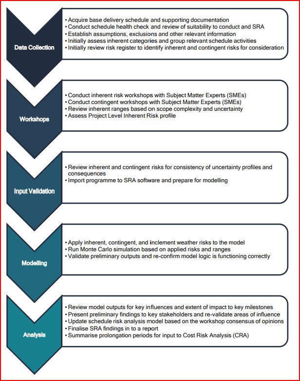
A rigorous QSRA follows a structured process. The diagram below shows a proven five-phase workflow used in practice on major infrastructure programmes:
Risk vs Uncertainty — Distinguishing the Two
The terms are often used interchangeably in practice, but they have distinct meanings in schedule risk analysis:
Merge Bias — Why the Schedule Underestimates Duration
One of the most important — and most underestimated — reasons for performing a schedule risk analysis is merge bias: the overall programme schedule duration will typically exceed the sum of the individual path durations, because of the way parallel paths merge at key programme events.
Wherever multiple parallel paths converge at a key event (preliminary design review, phase gate, product delivery, system integration), the timing of that event is controlled by the latest completing path. Any one of the merging paths can become critical. Because any path can be delayed, and the delayed path determines the merge date, the overall probability of delay at each merge point is higher than any individual path's probability of delay in isolation. A deterministic CPM schedule, calculated with single-point durations, will structurally underestimate the overall programme duration as a result.
Three-Point Estimates
The most common method for capturing duration uncertainty in an SRA is the three-point estimate: an optimistic (best-case), most-likely, and pessimistic (worst-case) duration for each activity or risk. The Monte Carlo simulation then randomly samples from a probability distribution fitted to these three points for each iteration.
A limitation of three-point estimates is that the individual risks affecting duration cannot be separately identified — an SME may be combining several threats and opportunities into a single range estimate. The result tells you how much contingency is needed, but not which specific risks are driving it. For targeted risk mitigation, the risk driver method is more powerful.
Risk Drivers — A More Powerful Approach
The risk driver method assigns specific identified risks to the activities they affect, with a probability of occurrence and a distribution of impact. Instead of expressing uncertainty as a duration range, duration uncertainty is derived indirectly from the risks that drive it.
How it works:
- A risk can be assigned to multiple activities — if the risk occurs in an iteration, it affects all assigned activities simultaneously
- An activity's duration can be influenced by multiple risks
- If a risk does not occur in a given iteration, the activity duration is unchanged for that iteration
- Correlation between activities is modelled naturally — if a risk fires, all affected activities are correlated through that risk
- Removing one risk at a time and re-running the simulation identifies each risk's individual contribution to schedule contingency — enabling targeted mitigation
In practice, the two methods are often combined: three-point estimates represent inherent uncertainty and estimating bias (the "unknown unknowns"), while risk drivers represent the identified, named risks from the register that can be mitigated.
Correlation Between Activity Durations
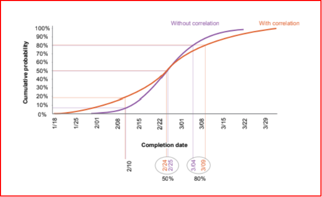
When two or more activities are influenced by the same external factor — the same technology assumption, the same contractor's productivity, the same design maturity — their durations will tend to move together. If that factor is unfavourable, all affected activities will tend to be longer; if favourable, shorter. This is positive correlation.
Without specifying correlation in the simulation, iterations where one activity goes long and another short are treated as equally plausible as iterations where both go long — which is inconsistent with the underlying reality. Specifying correlation ensures each iteration represents a coherent scenario.
Schedule Contingency
Schedule contingency is the buffer of additional time held by the programme manager to account for known risks and uncertainty. It represents the gap between the planned completion date (the last activity in the schedule) and the committed date (the date publicly promised to stakeholders).
Contingency = Pn date (from Monte Carlo) − deterministic schedule completion date. The target percentile (n) reflects the organisation's risk tolerance — typically P70 to P80 for major infrastructure.
Best practice is to hold contingency as a single activity immediately before the finish milestone. Dispersing contingency across multiple milestones throughout the schedule makes it harder to track, encourages teams to use it prematurely, and may hide total float on the critical path. Contingency should never be represented as a lag — lags have no descriptive name in the schedule and the associated contingency becomes invisible.
Total float is derived from network logic — it is the time an activity can slip before affecting the finish milestone. Contingency is derived from the schedule risk analysis — it is the time buffer the programme manager holds above the deterministic schedule to achieve a desired confidence level. They are fundamentally different quantities and should not be confused.
Contingency is held by the programme manager but can be allocated to contractors and subcontractors as needed. All allocations must go through formal change control — so that contingency consumption is tracked, monitored, and transparent. Subjecting contingency to change control prevents it being quietly absorbed by scope growth or inefficiency without being visible to management.
Prioritising Risks — The Tornado Chart and Risk Criticality
No programme can mitigate every risk. The SRA outputs provide two primary tools for prioritisation:
A bar chart ranking activities or risk drivers by their correlation with the project finish date — from highest impact to lowest. It identifies where the greatest risk exposure lies, but cannot by itself tell you which specific risk to mitigate first. The chart is the starting point for deeper investigation.
The percentage of Monte Carlo iterations in which an activity or milestone falls on the critical path. An activity with 85% risk criticality appears on the critical path in 85% of all simulated scenarios — even if its deterministic float appears comfortable. High-criticality activities demand close management attention.
To precisely rank individual risk drivers, remove one risk at a time, re-run the simulation, and record the change in the P80 date. The risk whose removal produces the greatest date improvement is the highest-priority risk for mitigation. Repeat iteratively to build the full prioritised list.
Collecting Unbiased Risk Data
The quality of QSRA outputs depends entirely on the quality of the input data. Risk interviews require rigorous management to prevent bias from corrupting the results.
Motivational bias occurs when interviewees feel that providing honest worst-case estimates will result in negative consequences — being labelled a troublemaker, being ostracised by the team, or contradicting management expectations. Risk workshops with authority figures present almost always produce compressed pessimistic ranges. To collect unbiased data:
- Guarantee anonymity and non-attribution for all SME input
- Conduct individual interviews without authoritative figures present
- Actively encourage interviewees to brainstorm genuine worst and best case scenarios
- Interview lower-level employees (who understand day-to-day task realities) as well as senior decision makers
- Allow interviewees to introduce risks beyond the existing risk register
Benefits of QSRA
Provides a statistical basis for schedule contingency decisions — replacing gut-feel buffer with a defensible, probabilistic analysis.
Pinpoints which risks have the most significant potential to delay the project, enabling focused, efficient risk management.
Quantified risk results demonstrate rigour and transparency to clients, financiers, and governance bodies — particularly on public sector programmes.
By identifying the highest-impact risks early, project managers can direct mitigation resources where they will have the greatest effect on schedule performance.
Challenges
QSRA requires a solid understanding of statistical methods, risk modelling concepts, and the specific software platform being used. Interpreting results correctly — and communicating them meaningfully to non-specialists — is a skill developed over years of practice.
The accuracy of QSRA outputs is entirely dependent on the quality of the input data. Biased, incomplete, or inconsistent risk data will produce misleading results that can actually damage decision-making by creating false confidence.
Specialist Monte Carlo simulation software (Safran Risk, Primavera Risk Analysis, @RISK, ARM) is required. The underlying CPM schedule must also be of sufficient quality to function as a valid simulation model — a flawed schedule produces a flawed risk model.
- QSRA quantifies schedule risk as a probability distribution of completion dates — not a single deterministic date
- The base case must be clearly defined before contingency can be meaningfully calculated
- Monte Carlo simulation runs thousands of iterations, randomly sampling durations, to build the S-curve
- Merge bias means CPM schedules structurally underestimate overall programme duration — SRA reveals the true risk
- Correlation widens the distribution and makes high-percentile commitment dates later — it matters for P70+ targets
- Schedule contingency ≠ total float — they are fundamentally different concepts
- SRA results are inputs to risk management decisions, not forecasts of how the project will actually unfold
Reference: U.S. Government Accountability Office. (2018). GAO Schedule Assessment Guide: Best Practices for Project Schedules. GAO-16-89G. Createspace Independent Publishing Platform.
SRA Quiz
Select the best answer for each question.
Q1. What is the primary objective of Schedule Risk Analysis?
Q2. Monte Carlo Simulation is a popular tool used in SRA for:
Q3. Which of the following is NOT a common technique used in Schedule Risk Analysis?
Q4. What is the difference between Schedule Risk Identification and Schedule Risk Assessment?
Q5. A project with a large buffer (float) in its critical path is generally considered:
Discussion & Scenario Questions
Q6. A construction project has identified a potential risk of material delivery delays. This risk could potentially delay several critical path activities. How would you approach this risk using Schedule Risk Analysis techniques? Briefly explain the steps involved in analysing the impact of this risk on the project schedule.
Q7. Discuss the advantages and limitations of using Monte Carlo Simulation for Schedule Risk Analysis. In your answer, consider the quality of input data, the interpretability of outputs, and how you would communicate the results to a non-technical project sponsor.