What is Schedule Risk Analysis?

What is Schedule Risk Analysis?

Quantitative Schedule Risk Analysis (QSRA) is a sophisticated technique used in project management to understand and quantify the uncertainty associated with the schedule of a project.

SQRA is a highly specialised field that is far more than just learning how to ‘drive’ Risk software. Interpreting the outputs from the ‘software’ is where knowledge and understanding is essential and typically based on many years of experience.

Opportunity (positive aspect of uncertainty) or Risk (negative aspect of uncertainty) should be considered and evaluated.

During the Planning phase of the Project, it should be clearly established what the Projects schedule strategy is. Ie. what is the base case for the schedule:

Explicit objectives are needed as the schedule contingency is assessed relative to the base case. If the base case is not known or understood, then it is challenging to effectively determine the contingency.

A historic norms strategy assumes average historical performance and is a strategy for mediocre performance at best.

SQRA goes beyond identifying potential risks by evaluating the probability and impact of these risks on the project’s completion date.

QSRA helps project managers make informed decisions by providing a statistical probability of project completion dates and identifying the key risk factors that might affect the schedule. This analysis is crucial for complex projects where timing is critical, and delays could have significant financial or operational impacts.

Process of QSRA

The QSRA process typically involves the following steps:

Benefits of QSRA

Challenges

In conclusion, Quantitative Schedule Risk Analysis is a powerful tool for managing and mitigating schedule risks in project management. It provides a more nuanced understanding of potential delays, enabling project managers to plan more effectively and increase the likelihood of project success.

SRA Curve & Tornado Chart

The SRA curve shows the probability of project completion over time. In this simplified example, the curve indicates that there’s a 60% chance the project will be completed by the end of Month 6 (on time).

However, the probability of completion increases to 80% by the end of Month 7, 95% by the end of Month 8, and reaches 100% by the end of Month 9, illustrating a clear risk of delay.

This visualization helps stakeholders understand the likelihood of meeting the project’s scheduled completion date and supports decision-making regarding risk mitigation and contingency planning.

Tornado Chart – Schedule Risk Impact

The Tornado Chart visually represents the impact of various risks on the project’s schedule, ranked from highest to lowest. In this scenario,

This chart is instrumental in prioritizing risk management efforts, focusing on mitigating the risks with the greatest potential impact on the project schedule.

Together, these visualizations provide a comprehensive view of the potential schedule risks a project faces, enabling more informed decision-making and effective risk management strategies.

Office, U. S. G. A. (2018, January 5). Gao Schedule Assessment Guide. Createspace Independent Publishing Platform.

Definition of Schedule Risk Analysis

A schedule risk analysis uses statistical techniques to predict a level of confidence in meeting a program’s completion date. This analysis focuses on uncertainty and key risks and how they affect the schedule’s activity durations. Because each activity has an uncertain duration that depends in part on uncertainties about effort and resources, the entire duration of the overall program schedule is also uncertain. Therefore, unless a statistical simulation is run, calculating the completion date from schedule logic and duration estimates in the schedule tends to underestimate the overall program critical path duration.

Estimates of activity durations should be viewed as forecasts based on the best information available at the time. Assumptions regarding resource availability and productivity, required effort, and availability of materials, among other things, allow for the determination of the most likely activity durations.

However, there is inherent uncertainty about the most likely duration estimate that can cause activities to shorten or lengthen.

Activity duration estimates include inherent uncertainty, estimating error, and, perhaps, estimating bias. For instance, if a conservative assumption about labour productivity was used in calculating the duration of an activity and during the simulation, a better labour productivity is possible, then the activity will shorten, at least for that iteration.

However, schedule underestimation is more pronounced when the schedule durations or schedule logic include optimistic bias. Activity durations and logic in a CPM schedule may be overly optimistic if there is pressure from the customer or instruction from management to finish earlier than the unbiased duration estimates imply.

Schedule Uncertainty and Risk

The terms risk and uncertainty are often used interchangeably, but they have distinct definitions in program risk analysis. Uncertainty refers to a situation in which little to no information is known about the outcome. A risk is an uncertain event that could affect the program positively or negatively. Stated another way, risk and its outcomes can be quantified in some definite way, while uncertainty cannot be defined because of ambiguity. In a situation that includes unfavourable and favourable events, the probability is that an unfavourable event will occur (a threat or harm) or that a favourable event will occur (an opportunity or improvement). Uncertainty and risk events may contain elements of both opportunity and threat. Schedule activity durations should account for both risk and uncertainty. Risk and uncertainty in scheduling refer to the fact that because activity durations are forecasts, there is always a chance that actual activity durations—and therefore scheduled start dates and finish dates—will differ from the plan. There will always be some aspect of the unknowable, and there will never be enough data available in most situations to develop a known frequency distribution of possible durations.

Risk events that can be listed and defined should be included in a program’s risk register in the form of threats and opportunities. Uncertainty arises because of the inherent variability in the actions of individuals and organizations working toward a plan. Uncertainty may also include estimating error and even systematic bias, such as when estimates are consistently optimistic. These events are often called “unknown unknowns.” As the program progresses, some uncertainties may be revealed or elaborated on and defined in the risk register as a threat or an opportunity. Prudent organizations recognize that uncertainties and risks can become better defined as the program advances and conduct periodic re-evaluations of the risk register.

As we describe in the following sections, threats and opportunities, as well as general uncertainty, can be incorporated and quantified to some degree using schedule risk analysis.

Merge Bias and Schedule Underestimation 

One of the most important reasons for performing a schedule risk analysis is that the overall program schedule duration may well be greater than the sum of the path durations for lower-level activities.

This is so partly because of schedule uncertainty and schedule structure. A schedule’s structure has many points where parallel paths merge that can cause the schedule to lengthen.

Merge points may include key program events such as preliminary design review, the beginning or ending of project phases, or product deliveries. The timing of these merge points is determined by the latest merging path.

Thus, if a required element is delayed, the merge event will also be delayed. Because any merging path can be risky, any merging path can determine the timing of the merge event.

Conducting a Schedule Risk Analysis

Schedule risk analysis relies on statistical simulation to randomly vary the following:

• activity durations according to their probability distribution;

• threats and opportunities according to their probability and the distribution of

their effect on affected activities if they were to occur; and • the existence of a risk or probabilistic branch.

The objective of the simulation is to develop a probability distribution of possible completion dates that reflect the program plan (represented by the schedule) and its quantified uncertainties and risks. From the cumulative probability distribution, the organization can match a date to its degree of risk tolerance. For instance, an organization might want to adopt a program completion date that provides a 70 percent probability that it will finish on or before that date, leaving a 30 percent probability that it will overrun, given the schedule and the risks as they are known and calibrated. The organization can thus adopt a plan and promise completion on dates that are consistent with its preferred level of confidence in the overall integrated schedule. A schedule risk analysis can provide valuable information to senior decision makers.

Risk analysis should not be focused solely on the deterministic critical path—that is, the critical path as defined by the initial or current set of inputs in the schedule model.

Because the durations of activities are uncertain, with risk considered, any activity may potentially affect the program’s completion date. Hence, the path that is most likely to determine the finish date is uncertain.

If the analysis is to be valid, the program must have a good schedule network that clearly identifies the work that is to be done and the relationships between detailed activities.

The schedule should be based on a minimum number of justified date constraints. It is important to represent all work in the schedule, because any activity can become critical under some circumstances.

Complete and correct schedule logic that addresses the logical relationships between predecessor and successor activities is also important. The analyst needs to be confident that the schedule will automatically calculate the correct dates and critical paths when the activity durations change, as they do thousands of times during a simulation.

If time or resources are insufficient to simulate the full program, or if detail in the future is unclear, perhaps because of rolling wave planning, the simulation can be performed with a summary version of the schedule. The summary schedule is a condensed form of the schedule that rolls detail activities into long-duration activities. By reducing the number of activities in the schedule, analysts reduce the time spent collecting data about and assigning risks and probability distributions to detail activities.

However, if a summary schedule is used for a schedule risk analysis, it is important that the schedule show enough detail to yield practical results. A summary schedule that is condensed too much will not convey the effort in very long activities, the activities that should have assigned risks, or how total float is distributed among key activities and milestones.

For example, activities in the summary version of the schedule should show critical hand-offs. If an activity is 4 months long but a critical hand-off is expected halfway through, the activity should be broken down into separate 2-month activities that logically link the hand-off between activities.

Finally, condensing the schedule may hide merging paths. As discussed in the previous section, merging paths are the source of much risk.

After the risk information is developed, the statistical simulation is run and the resulting cumulative distribution curve, the S curve, displays the probability associated with the range of program completion dates. The results of risk analysis are best viewed as inputs to program management rather than as forecasts of how the program will be completed. The results indicate when the program is likely to finish without the program team’s taking additional risk mitigation steps. The high-priority risks can be identified and used to guide further risk mitigation action.

A schedule risk analysis may show that a given schedule has more risk than is acceptable.

In this case, a review of the activities, dependencies, and network might help derive a shorter schedule. In some cases, the scope may need to be reduced. However, the initial estimates of effort and duration should not be changed without sufficient justification.

Changing durations simply because an earlier finish date is preferred is likely to increase the risk of delaying a project.

Collecting Anonymous and Unbiased Risk Data

A schedule risk analysis requires the collection of program risk data. Risk data should be derived from a quantitative risk assessment and should not be based on arbitrary percentages or factors. A risk assessment is a part of the program’s overall risk management process in which risks are identified and analysed and the program’s risk exposure is determined. As risks are identified, risk-handling plans are developed and incorporated into the program’s cost estimate and schedule, as necessary.

Risk data can be collected in the form of three-point durations or by using the risk driver approach, to be described in the next section. The three-point estimates represent inherent uncertainty, estimating error, and perhaps estimating bias, while risk drivers represent identified risk events with probabilities as well as the likely effect if they occur.

Regardless of which type of risk analysis is performed, it is essential that subject matter experts (SME) be interviewed who are directly responsible for or involved in the workflow activities.

Estimates derived from interviews should be formulated in a consensus of knowledgeable technical experts and should be coordinated with the same people who manage the program and its risk mitigation watch list.

Employees involved in the program from across the entire organization should be considered for interviewing. Lower-level employees have valuable information on day-to-day tasks in specific areas of the program, including their insight into how individual risks might affect their workflow responsibilities.

Managers and senior decision makers have insight into all or many areas of the program and can provide a sense of how risks might affect the program as a whole.

The starting point for the risk interviews is the program’s existing risk register. Interviewees are asked to provide their opinion on threats and opportunities and should be encouraged to introduce additional risk events that are not on the risk register.

If unbiased data are to be collected, interviewees must be assured that their opinions on threats and opportunities will remain anonymous. They should also be guaranteed non attribution and should be provided with an environment in which they are free to brainstorm on worst and best case scenarios.

It is particularly important to interview SMEs without an authoritative figure in the room to avoid motivational bias.

Motivational bias is a source of bias that arises when interviewees feel threatened (whether justifiably or non-justifiably) if they give their true thoughts about a program.

This threat is typically from fear of being punished by someone in authority. Most commonly, interviewees are labelled trouble makers or are ostracized from the team if their worst case scenario is worse than management’s opinion.

Risk workshops may exhibit social and institutional pressures to conform, perhaps to get consensus or to shorten the interview session. The organization may greatly discourage introducing a risk that has not been previously considered, particularly if the risk is sensitive or may negatively affect the program.

If an interviewee is accompanied by someone, risk analysts cannot guarantee that the interviewee’s responses are unbiased.

Once the distributions have been established, a statistical simulation (typically a Monte Carlo simulation) uses random numbers to select specific durations from each activity probability distribution, and a new critical path and dates are calculated, including major milestone and program completion dates.

The Monte Carlo simulation continues this random selection thousands of times, creating a new program duration estimate and critical path each time. The resulting frequency distribution displays the range of program completion dates along with the probabilities that activities will occur on these dates.

Three-point duration risk analyses, an acceptable method of conducting SRAs, are widely used. However, a disadvantage of using three-point duration ranges to represent all the risk in an analysis is that probability distributions for durations derived from risk interviews cannot be attributed to individual risk events.

Interviewees may be combining any number of threats and opportunities in their single best case and worst case estimates.

For example, a construction manager may suggest a worst-case scenario of 6 days to install drywall. However, the delay may be caused by lack of materials, poor labour productivity, poor weather, last-minute design changes, or some serial combination of all four risks. It is also possible that the SME has increased the pessimistic duration estimate to account for general uncertainty, in effect accounting for “unknown unknowns.”

The result of the three-point duration SRA is a recommended amount of schedule contingency that covers both quantified risks and some level of uncertainty but gives no indication of which risks are most likely to affect the schedule.

Schedule Risk Analysis with Risk Drivers

A second way to determine schedule activity duration uncertainty is to analyse the probability that risks from the risk register may occur and what their effect on schedule activities will be if they do occur.

With this approach, a probability distribution of the risk impact—expressed as a multiplicative factor—on the duration of activities in the schedule is estimated and the risks are assigned to specific activities in the schedule. If a risk does not occur in an iteration, then the scheduled duration does not change for that activity. In this way, activity duration risk is estimated indirectly by the root cause risks and their assignments to activities.

A risk can be assigned to multiple activities and the durations of some activities can be influenced by multiple risks. This risk driver approach focuses on risks and their contribution to time contingency as well as on risk mitigation. The risk driver method can be used to examine how various risks may affect the house construction schedule.

We can suspect that the biggest risk in the construction schedule involves design and that the plan may be too aggressive in assuming that the design will be completed early. Moreover, late or defective materials and changes by the owner are also likely to affect the schedule.

In addition to including discrete threats and opportunities, we can include risks that represent ambiguity about the future. The existence of these ambiguities is known (their likelihood is 100 percent) but their effects are unknown.

For example, we know that the productivity of labour will affect the duration of many activities, but whether the overall effect is positive (an opportunity) or negative (a threat) is unknown.

We can also include some element of general uncertainty. For example, we know that natural variability surrounds each of our duration estimates, so we include an uncertainty to represent a global estimating error.

By combining the two methods, three-point estimates may be used to represent bias and uncertainty, while risk drivers are used to represent identifiable risk events that may be mitigated.

Prioritising Risks

No program can mitigate all risk and uncertainty. Some risks may be highly probable yet cause a relatively small delay to the finish date. Conversely, a risk may potentially delay the program a long time but be highly unlikely to ever occur. In addition, it is impossible to fully mitigate uncertainty because of its inherent ambiguity.

Therefore, regardless of the method used to examine schedule activity duration uncertainty, it is important to identify the risks that contribute most to the program schedule risk. These risks can then be targeted for mitigation strategies.

Sensitivity measures reflecting the correlation of the activities or the risks with the final schedule duration can be produced by most schedule risk software.

The duration sensitivity chart identifies activities and paths that tend to be associated with project risk. 

Risk analysis should also identify the activities that most often ended up on the critical path during the simulation, so that near risk-critical path activities can be identified and closely monitored. Risk criticality represents the percentage of simulation iterations that an activity or milestone is on the critical path.

The activities most likely to be on the critical path may not be the most risky themselves. The activities may be critical because they are appearing on a path

whose criticality is driven by some risk affecting other activities.

Sensitivity indexes and correlation measures are useful starting points for assessing the possible magnitude of realized risks, but they have limited use in prioritizing risks.

Thus, while the chart is useful for indicating where risk is the greatest, it cannot be used to identify specific risks for mitigation.

If the risk drivers method is used, the risks can be prioritized by their effect on the risk of finishing on time and their share of required contingency. If one risk at a time is removed and the Monte Carlo simulation is rerun, the contribution of each risk to the required contingency can be calculated at any percentile.

The general process is to:

• Run the SRA using all risks and uncertainties. Record the finish date at the desired percentile—for example, 80 percent.

• Remove a risk and run the SRA again. Compare the 80th percentile date with the date of the full model. The difference in the two dates is the expected contribution (or days saved) of the removed risk.

• Replace the risk, remove the next risk, rerun to the SRA, and again compare the 80th percentile date to the date from the full SRA simulation and calculate the

difference in days.

Continue removing risks and uncertainties one by one; the risk with the highest contribution in days is the most important risk.

To identify the next most important risk, the most important risk identified above is removed from the model and the process is repeated

As the risks are removed and the next most important risks are identified, a prioritized list of risks and uncertainty can be created.

Correlation

Other capabilities are possible once the schedule is viewed as a probabilistic statement of how the program might unfold. One that is notable is the correlation between activity durations.

Positive correlation is when two activity durations are both influenced by the same external force and can be expected to vary in the same direction within their own probability distributions in any consistent scenario.

Correlation might be positive and fairly strong if, for instance, the same assumption about the maturity of a technology is made to estimate the duration of design, fabrication, and testing activities or the contractor’s productivity affecting multiple activities that have been bid.

If the technology maturity is not known with certainty, it would be consistent to assume that design, fabrication, and testing activities would all be longer or shorter together.

Likewise, if a particular trade is relatively unproductive in the house construction

example, we may expect all activities associated with that trade to be delayed to some degree.

Without specifying correlation between these activity durations in simulation, some iterations or scenarios would have some activities that are thought to be correlated go long and others short in their respective ranges during an iteration.

This would be inconsistent with the idea that they all react to the same assumptions about technology maturity or trade productivity.

Specifying correlations between related activities ensures that each iteration represents a scenario in which their durations are consistently long or short in their ranges together.

Because schedules tend to add durations (given their logical structure), if the durations are long together or short together, there is a chance that projects will be very long or very short.

Correlation affects the low and high values in the simulation results. This means that the high values are even higher with correlation and the low values are even lower, because correlated durations tend to reinforce one another down the schedule paths.

In practice, if the organization wants to focus on the 80th percentile, correlation matters; correlation does not matter as much around the mean duration from the simulation.

Figure 2 shows the effect of adding correlation between activity durations in the three point risk simulation for the house construction schedule. In this example, 90 percent correlation was added between activities that are related trades. While the 90 percent correlation is high (correlation is measured between –1.0 and 1.0), there is often no actual data on correlation, so expert judgment is often used to set the correlation coefficients.

Assuming this degree of correlation, we get the result shown in figure 7. Notice that the correlation has widened the overall distribution. The 50th percentile is nearly the same in both cases, February 25 without correlation and February 24 with correlation. However, the 80th percentile increases by one workweek, from March 4 to March 9, when correlation is added.

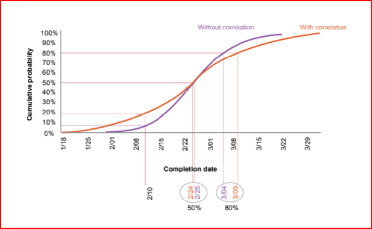
Figure 2

Using three-point estimates for activity durations requires estimating correlation coefficients, often in the absence of historical data. Inconsistent correlation matrices often result in this pairwise setting of correlation coefficients.

In the risk driver method, assigning a risk to multiple activities causes them to be correlated, because if the risk occurs on one assigned activity during the simulation, it occurs on all the assigned activities. If there are also some risks on one activity but not another, correlation will be less than 100 percent.

Modelling correlation with risk drivers avoids the difficult task of estimating a number of pairwise correlations.

Schedule Contingency

A baseline schedule includes margin or a reserve of extra time, referred to as schedule contingency, to account for known and quantified risks and uncertainty.

The contingency represents a gap in time between the finish date of the last activity (the planned date) and the finish milestone (the committed date).

When schedule contingency is depicted this way, a delay in the finish date of the predecessor activity results in a reduction of the contingency activity’s duration. This reduction translates into the consumption of schedule contingency.

Schedule contingency should be calculated by performing a schedule risk analysis and comparing the schedule date with that of the simulation result at a desired level of certainty.

For example, an organization may want to adopt an 80 percent chance that its program will finish on time or earlier. The amount of contingency necessary would be the difference in time between the 80th percentile date from the cumulative distribution and the date of the deterministic finish date in the schedule.

For some programs, the 80th percentile is considered a conservative promise date. Other organizations may focus on another probability, such as the 65th or 55th percentile.

However, because schedule distributions tend to be right skewed (that is, the program has a greater tendency to finish late than early), the mean of the distribution tends to be larger than the 50 percent confidence level.

The 55th or 65th percentiles are not as certain as the 80th percentile and may expose the program to overruns if they are adopted. Factors such as project type, contract type, and technological maturity affect each organization’s determination of its tolerance for schedule risk.

Schedule contingency or reserve is held by the program manager but can be allocated to contractors, subcontractors, partners, and others as necessary for their scope of work.

When contingency needs to be allocated, a formal change process should be followed.

Subjecting schedule contingency to the program’s change control process ensures that variances can be tracked and monitored and that the use of contingency is transparent and traceable.

Schedule contingency may appear as a single activity just before the finish milestone or it may be dispersed throughout the schedule as multiple activities before key milestones or allocated to different phases of the project (Design, Procurement, Installation/Construction, Commissioning).

For example, it might be appropriate to plan a contingency activity before the start of a key integration activity that depends on several external inputs to ensure readiness to start. It is preferable that contingency be held as one activity just before the finish milestone for several reasons.

In general, apportioning contingency in advance to specific activities is not recommended because risks that will actually occur and the magnitude of their effects are not known in advance. In addition, dispersing contingency to specific key milestones may cause its consumption prematurely or superfluously.

Contingency that is dispersed throughout the schedule is less visible and may be harder to track and monitor. Dispersion may also encourage team members to work toward late dates rather than the expected early dates.

By aggregating contingency, everyone on the project will be working to protect the schedule contingency as a whole, not simply their own portions. Finally, if contingency activities are dispersed within the schedule network, care must be taken that the contingency activities do not affect total float and, therefore, critical path calculations.

Contingency activities should not become critical because no resources or scope are associated with them and they cannot practically delay a successor activity.

Regardless of whether contingency is captured at the end of the schedule or just before key milestones, representing it as activities will help ensure that the schedule is not hiding potential problems.

Contingency can also be quickly identified and zeroed out before schedule health measures are calculated or an SRA is conducted if it is represented as activities.

Finally, schedule contingency should not be represented as a lag between two activities. Lags have no descriptive name in schedules and the associated contingency may become lost within the network logic.

Notice that contingency is not the same as total float. Total float is the amount of time by which an activity can be delayed before it affects the finish milestone.

Total float is directly related to network logic and is calculated from early and late activity dates. Schedule contingency, in contrast, is determined by a schedule risk analysis.

A schedule risk analysis compares the schedule date with that of the simulation result at a desired level of certainty and is calculated by quantifying uncertainties and risks that may affect the finish date.